
Biological fermentation is complex. It includes microbial growth, metabolic activities and product synthesis. Mathematical models are very important tools. They help optimize these processes. They help predict working performance. They help reduce production costs. These Mathematical models change the complex biology of fermentation into clear relationships.
These Mathematical models help researchers and engineers. They can do fewer tests during process development. They can use less energy. They can keep product quality stable when they scale up production. Scaling up means moving from small lab shake flasks to big industrial bioreactors. Using Mathematical Models makes scaling up more reliable.
Classification by Modeling Principles
01 White-box models (mechanistic models)
These Mathematical Models use the biochemical rules of fermentation systems. They use differential equations. These equations show the dynamic links between microbial growth, substrate consumption and product formation. They are based on basic biological knowledge. This knowledge includes enzyme kinetics, metabolic pathway rules and mass transfer basics. These Mathematical Models work well in similar fermentation systems.
One common of these Mathematical Models example is the Monod equation: μ = μₘₐₓ[S]/(Kₛ + [S]). μ is the specific growth rate. μₘₐₓ is the maximum specific growth rate. [S] is substrate concentration. Kₛ is the half-saturation constant. This equation shows how microorganisms grow when nutrients are limited. It shows the hyperbolic relationship between substrate concentration and specific growth rate. It is very useful for industrial fermentation. These fermentations are often limited by carbon or nitrogen.
These Mathematical Models have clear physical meanings. They need a lot of test data to set parameters. They also simplify complex metabolic pathways. For example, they ignore interactions between secondary metabolites. This can cause wrong predictions. These wrong predictions happen in high-cell-density or mixed-strain fermentations.
02 Black-box models (empirical models)
These models only use input and output data of the fermentation process. They build relationships between variables. They use statistical methods or machine learning tools. These tools include artificial neural networks, support vector machines and random forests.
These models work well in some fermentation situations. The internal mechanisms are not fully known in these situations. Or variables are closely connected. Examples include mixed microbial community fermentation. Another example is fermentation with complex materials. These materials include lignocellulosic biomass.
Response surface models (RSM) are a good example of these Mathematical Models. They are often used with test design (DOE) methods. These methods include Box-Behnken or central composite design. They can optimize medium parts and process parameters quickly. They only need a few tests. Process parameters include pH, cultivation temperature and aeration rate.
These models have one big problem. They cannot explain the biology behind the process. They only predict results. They do not explain why a group of parameters works. So they are less flexible. They work worse when strains or raw materials change.
03 Grey-box models (hybrid models)
These Mathematical Models combine mechanism-based and data-based methods. They balance biological meaning and prediction accuracy for fermentation processes.
For example, we can merge metabolic flux analysis (MFA) with kinetic equations. This keeps some mechanism explanations. It also improves prediction accuracy with data calibration.
We can also add machine learning parts to a basic mechanism model. This fixes unmodeled problems in fermentation. These problems include cell lysis or foam formation.
These Mathematical Models are used more often in industrial bioprocesses. Pure mechanism models cannot fully show real fermentation complexity in these processes.
Classification by Spatiotemporal Characteristics
01 Homogeneous and heterogeneous models
Homogeneous models see the bioreactor as one single phase. An example is liquid. They think substrates, microbial cells and products are spread evenly. Mathematical Models are good for well-mixed fermentation systems. Examples include stirred-tank bioreactors (STRs) with high stirring speed.
Heterogeneous models are different. They tell gas, liquid and solid phases apart in the reactor. Examples include oxygen mass transfer in aerobic fermentation. Another example is solid substrate breaking down in corn stover-based bioethanol production. They also consider concentration gradients of substances inside the reactor.
These Mathematical Models are very important. They are important when scaling up fermentation. Mass transfer problems become big issues at that time. One example is low oxygen in high-cell-density cultures.
Dynamic and static models
Dynamic mathematical models use differential equations to track how fermentation variables change over time. Examples are biomass growth curves in batch fermentation or substrate consumption patterns in fed-batch processes. This enables real-time monitoring and control of the fermentation process. Static Mathematical Models are different. They apply to steady-state fermentation (e.g., input-output material balance in continuous fermentation). They are often used to optimize long-term production efficiency. For instance, they help determine the best dilution rate for chemostats. This maximizes product yield.
Classical Kinetic Models for Fermentation
Microbial Growth Kinetic Models
Mathematical Models in this category form the backbone of microbial growth prediction.
Monod equation
It describes the specific growth rate (μ) of microorganisms when substrates are limited. Industrial microbes like Escherichia coli and yeast often use it in fermentation. This fermentation is for biopharmaceuticals, biofuels and industrial enzymes. This is one of the most widely used Mathematical Models.
Andrews equation
This equation includes a substrate inhibition term (μ = μₘₐₓ[S]/(Kₛ + [S] + [S]²/Kᵢ), where Kᵢ is the inhibition constant). It is suited for fermentation scenarios. In these scenarios, high substrate concentrations inhibit microbial growth. Examples are ethanol’s toxic effect on yeast in alcoholic fermentation, or high glucose levels suppressing microbial metabolism in lactic acid production.
Logistic equation
It is used to fit the S-shaped microbial growth curve (X(t) = X₀K/(X₀ + (K – X₀)e⁻ᵣᵗ)). Here, X(t) is biomass at time t, X₀ is initial biomass, K is environmental carrying capacity, and r is intrinsic growth rate. This model has successfully predicted biomass concentration in processes. An example is catalase production by Aspergillus niger. In this process, microbial growth is limited by space or nutrient availability.
Product Formation Kinetic Models Mathematical Models in this category form the backbone of microbial growth prediction.
Luedeking–Piret equation
It links product formation to microbial biomass growth (dP/dt = αdX/dt + βX, with α as the growth-associated coefficient and β as the non-growth-associated coefficient). This classifies fermentation products into two types. The first type is growth-associated products (e.g., lactic acid). Their formation ties closely to energy metabolism during microbial cell division. The second type is non-growth-associated products (e.g., penicillin and other antibiotics). They are mostly synthesized during the microbial stationary growth phase.
Modified Gompertz model
This model tracks how fermentation metabolites (e.g., citric acid, glutamic acid) accumulate over time. It has key parameters. These parameters include lag phase length, maximum product formation rate and final product concentration. It can be combined with the extended Kalman filtering algorithm. This combination can estimate fermentation process states in real time. It supports adaptive control of operations. An example is adjusting feeding rates to keep product synthesis in optimal condition.
Kinetic Models for Complex Fermentation Scenarios
Multi-substrate inhibition model
This model accounts for both glucose and fermentation product inhibition in ethanol production. The production uses sweet potato hydrolysate. It addresses key technical challenges. These challenges are utilizing mixed sugars (e.g., glucose and xylose) and dealing with product toxicity in fermentation. It is solved via the Runge–Kutta method. This is a numerical integration technique. It is commonly used for solving ordinary differential equation systems in fermentation kinetic studies. Complex Mathematical Models like this one require numerical methods.
Temperature-coupled kinetic model
It adds temperature variables to batch bioreactor systems. It optimizes fermentation control system design. Examples of design are heating and cooling strategies. Temperature directly impacts enzyme activity, microbial growth rate and metabolite stability. This model quantifies these effects. It maintains an optimal fermentation temperature profile. This is especially critical for producing heat-sensitive products. Examples are recombinant proteins and probiotics. These Mathematical Models connect temperature with fermentation performance.
Major Technological Breakthrough!
Evo2 – The World’s Largest Biological Large Model Launches Officially!
This advanced model can accurately predict all types of gene mutations and their corresponding genetic coding sequences! (In-depth Comprehensive Analysis)
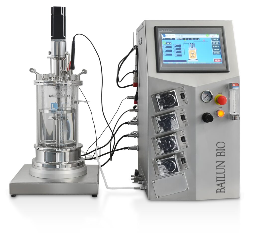
About Bailun
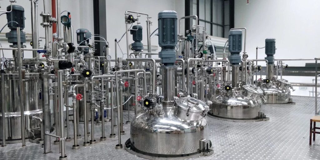
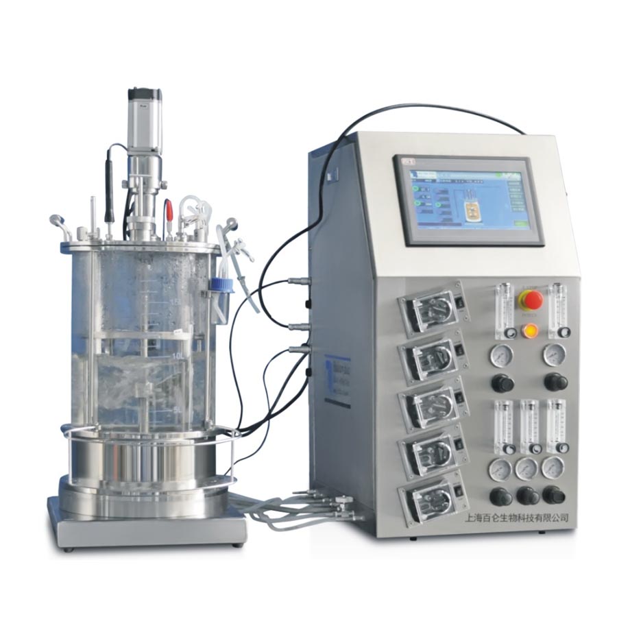
Bailun has rich experience manufacturing various bioreactors and pressure vessels. These include stirred-tank, airlift and fixed-bed designs. They are customized for microbial fermentation, cell culture and enzyme production. Our professional team covers fields. These fields are bioreaction engineering, fermentation technology, mechanical engineering and automation control. We have deep expertise in integrating mathematical models into fermentation process design. We help clients build mathematical models-based control systems.
These systems boost production stability and reliability. Our R&D and technological capabilities stand at the forefront in China. We are a manufacturer and factory with strong competitiveness. Our core service advantages are as follows:
Customization Services: We provide personalized optimization for bioreactor structure, agitation systems, monitoring modules and control programs. The optimization is based on customers’ process requirements. It matches the specific needs of cell expansion and differentiation for cultivated meat exactly. We use Mathematical Models to guide each customization step.
GMP / CE Certification: All equipment follows international standards strictly. This ensures products meet food safety and industry regulatory requirements. It also lowers market entry barriers. Our Mathematical Models help verify that equipment operates within certified parameters.
Turnkey Solutions: We offer full-process services. These services cover process design, equipment manufacturing, on-site installation, commissioning and personnel training. This shortens project implementation time greatly. It also reduces operational difficulty for customers. We apply Mathematical Models to every stage of the turnkey solution.
Cost Advantage: We have a mature supply chain. We also have large-scale production capacity. These support us to provide cost-effective equipment and services. We also ensure product quality and technological advancement. Contact Us